Area Between Curves
Step-By-Step Explanation
Step-by-step explanations to three examples that show how to find the area between two curves, or functions, are given below.
Example 1: Find the area under a sine function.
-
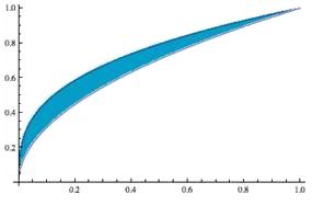
Example 2: Find the area between the functions
 and
and  .
. -
Example 3: Find the area "trapped" between two intersecting parabolas.
Example 1
| Figure | Problem | |
|---|---|---|
|
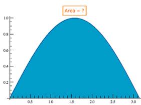
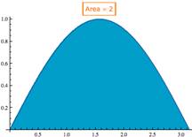
This example is a review of the process you learned in your first calculus course. Find the area under the first "hump" of the sine function. The graph shows sin(x) graphed on the interval [0, π] with the desired area shaded blue. |
|
| Step | Equation | Explanation |
| 1 | The area is given by the definite integral on the interval [0, π]. | |
| 2 | 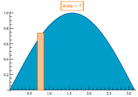 |
It is important to visualize the approximating rectangles. Recall from Calculus I that the integral used to find the area equals the limit of the sum of the areas of the approximating rectangles. It is not necessary to draw in all of the approximating rectangles; a single representative rectangle should help set up the problem. Recall that the area of a rectangle is its width times its length, where the width, dx, is along the x-axis and the height is along the y-axis, and is given by the value of the function f(x) = sin(x) for this example. |
| 3 | To solve the integration problem, we need the antiderivative of sin(x), which is –cos(x). |
|
| 4 | The area (the definite integral) is this antiderivative evaluated at the limits of integration. Evaluating and summing gives an area of 2. |
|
5 |
|
Thus, the area under the first "hump" of the sin(x) curve is 2 (square units). |
Example 2
| Figure | Problem | |
|---|---|---|
|
Find the area between the functions |
|
| Step | Equation | Explanation |
| 1 | The area is given by the definite integral of the absolute value of the difference in the functional values on the interval [a, b]. Note two things here:
|
|
| 2 | Solve |
Let's determine a and b first. A graph is helpful here but not required. The area is "trapped" in a region between the intersections of the curves; thus, to find a and b we need to determine the x values, where
or
|
| 3 |
Thus, x = 0 and x = 1 are the only solutions. That is, a = 0 and b = 1. |
By inspection and the graph, we can see that x = 0 and x = 1 are solutions, but let's show this algebraically and show that they are the only solutions. Solving,
Raise both sides of the equation to the 6th power. (Why the 6th power? Six is the least common multiple of 2, the square root, and 3, the cube root. Thus, raising both sides of the equation to the 6th power will remove both radicals.) |
| 4 | 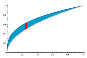 |
Again, visualize a rectangle that would be in the approximation to the area. Again, the width of that rectangle is dx, but the length is the y distance between the functions, that is,
This will always be positive if we subtract the lower value from the upper one. So, which curve is the upper one? Checking a graph or a calculator, on the interval (0, 1),
|
| 5 |
|
Now replace the absolute value with the positive difference of the functions. |
| 6 |
|
Rewrite the radicals as fractional exponents and find the antiderivatives. |
| 7 |
|
Do the evaluation (which is 0 for x = 0). |
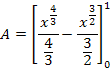
| 8 | Thus the area is |
|
A Diversion |
||
| 4a | 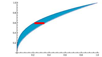 |
In step 4, you might have asked whether the rectangle must be "vertical." In fact, no, we could use horizontal rectangles to do the approximation. Notice that by doing so, the width becomes dy and the length is a difference in x values, so the integral needs to be written with respect to y. |
| 4b | Note that a and b are values along the y-axis, and that the function must be written in terms of y to perform the integration. (Also, note that because the functions are one-to-one on [0, 1], this can be done!) |
|
| 4c |
|
To remove the absolute value, the right values of x are greater, so xf is now associated with the square root function and xg with the cube root function. Solve the values and functions in terms of y. |
| 4d |
|
Note that the integral is now in terms of the y variable. Thus, we find the antiderivatives with respect to y. |
| 4e |
|
Simplifying the fractions results in the same area we obtained in our calculation in step 8, above. |

Example 3
| Figure | Problem | ||
|---|---|---|---|
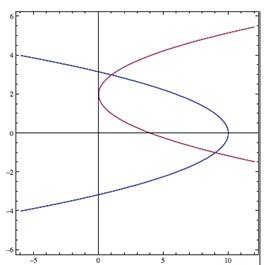 |
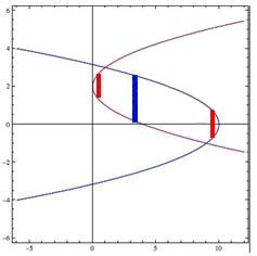
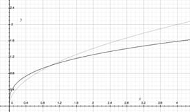
Find the area "trapped" between the implicit functions (It is left as an exercise for you to (1) identify which graph is which function, and (2) shade the trapped area.) |
||
| Step | Equation | Explanation | |
| 1 |
|
If we draw in some vertical rectangles, we see that sometimes the upper value is on one function and the lower value is on the other function (larger blue rectangle), but sometimes both values are on the same graph (smaller red rectangles). The calculations can still be done, but they are much more difficult than necessary. So we'll try a different approach. |
|
| 2 |
|
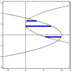
Let's try horizontal rectangles. Now, we see that no matter what the y value is, the horizontal rectangles are bounded by both graphs. This will make the calculation easier. Note that the width of these rectangles will be dy, and the length will be the difference in the x values. First, we must find the limits of integration, a and b, from the intersection points of the graphs. |
|
| 3 |
and Hence,
That is, a = –1 and b = 3 |
Solve each equation for x and set them equal to each other. Note that there are only two solutions (two intersection points), so there are no other "trapped" areas. We could find the x values associated with these y values, but it would be unnecessary work because we are integrating with respect to y. |
|
| 4 | We must determine which curve has the greater x values by examining the graphs or the function (x) values. We can see that the right-hand boundary, the graph |
||
| 5 |
|
Thus, we can set up the integration and simplify. (Notice that we have already done this work above, when finding the intersections.) |
|
| 6 |
|
Find the antiderivatives. |
|
| 7 |
|
Do the evaluation. |
|
| 8 |
|
(Of course, this is |
|