Area Between Curves
Summary
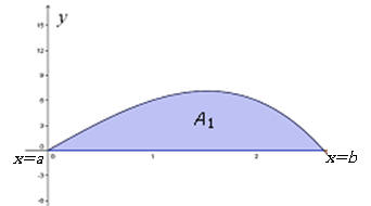
In Calculus I, you learned that the definite integral of a positive function on an interval [a, b] represents the "area under the curve" of the function. That is, it is the area under the graph of the function above the x axis between x = a and x = b. See area A1 in figure 1.
Figure 1
Area Under a Curve
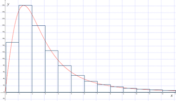
This area is calculated as the limit, if it exists, of a sum of the areas of approximating rectangles with width Δx along the x-axis and with lengths (heights) as a function value. The limit is taken as the number of these rectangles increases and their width decreases (that is, the width approaches zero). Although the heights of these rectangles can be chosen in a number of ways (function values at the left endpoint of the rectangle, right endpoint, etc.), in the limit, these methods are equivalent and result in the same value for the area.
In figure 2, each rectangle is chosen with its width along a subinterval of the x-axis and its height given by a function value on that subinterval.
Figure 2
Rectangles Approximating the Area Under a Curve
Note that the Fundamental Theorem of Calculus states that this limit process can be avoided—that, in fact, the definite integral (and area) can be evaluated by finding the antiderivative of the integrand and evaluating it at the endpoints (the limits of integration). This makes the evaluation process simpler, provided you can find the antiderivative.
It is important to keep the limit process in mind, especially when setting up the rectangles, because it can help you solve the problem. In fact, integration problems are really a matter of adding up small quantities (for example, the areas of rectangles when finding area), so identifying these quantities will define the integrand and enable you to solve the problem.
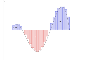
Also, remember that if the function is not positive on the interval of integration, the negative functional values will lead to "negative areas" that can subtract from the positive areas (see figure 3). That is, the definite integral gives the area only if these negative regions are made positive. Mathematically, this is done by using the absolute value of the function.
To solve the integral, the absolute value expression must be replaced by a positive difference. To do this, we must determine which regions are negative and make them positive by properly taking their difference to replace the absolute value.
Figure 3
Positive and Negative Areas of a Function
For example, in figure 4, the area "under" the sine curve—actually, between the curve and the x-axis on the interval [0, 2π]—is 4 square units; but the indefinite integral evaluates to zero. To calculate the area, we must determine the "negative regions" and take their absolute value (see figure 4 and associated equations).
|
Figure 4
|
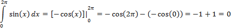
The graph shows the sine curve from x = 0 to x = 2π. The definite integral over this interval is,
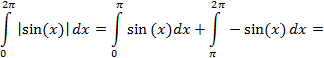
However, the area is given by,
|
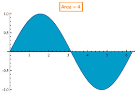
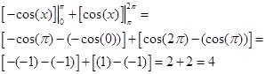
Note that the negative region had to be identified to apply the definition of the absolute value and make this region positive.
Now let's generalize the area problem from "under the curve" to "between the curves," where the curves can be two or more function graphs. For example, if f(x) and g(x) are two continuous functions defined on the interval [a, b], then the area between them (see figure 5) is defined as,
|
Figure 5
|
The absolute value in this formula makes it mathematically expedient to state; but in practice, to evaluate the integral, the "positive" and "negative" regions must be determined. That is, we must determine which function is "higher" (of greater value) than the other on the given interval.
The problem can be further complicated if the graphs cross one or more times on the interval.
In figure 6, the orange and yellow regions show where the functions cross or intersect, so each of these regions would result in a separate integral calculation that would sum to the true area. Also notice that although the function values can be negative, the difference of the functions is still positive when one function is above the other. To determine this difference, it is good to go back to thinking in terms of the rectangles that would be used to set up the integration. Let's examine this in more detail. |
|
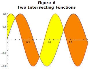
Figure 7
|
In figure 7, approximating rectangles (blue vertical lines) assist setting up the integration to properly define the differences in the functions. Note how the intersections (x1, x2, and x3) divide the region. We have placed four narrow blue rectangles in the graph. The leftmost one in the yellow region A1 has its upper edge on the graph of f(x) and its bottom edge on g(x). The next rectangle, in the orange region A2, has its upper edge on g(x) and lower edge on f(x). Thus, to calculate the absolute value and hence the area in region A1, we need to subtract: the upper value, f(x), minus the lower value, g(x). That is,
In region A2, we need to subtract g(x minus f(x), because the g(x values are the upper values; that is,
|
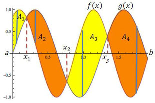
So to calculate the total area, we must determine the regions A1, A2, A3, and A4, and in particular, the values x1, x2, and x3, where the functions intersect. Stated mathematically in terms of the integration,
![]()
![]()
So our simple problem is starting to look more complicated. Our question now is, how do we find the values x1,
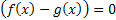
x2, and x3 of the intersections? This is the standard algebra problem of solving
(![]() ) for x, or stated more mathematically,
of finding the roots or zeros of (
) for x, or stated more mathematically,
of finding the roots or zeros of (![]() ).
This latter statement is useful when the functions are nonlinear and finding the zeros may be difficult or impossible analytically.
In those cases, we may want to use a numerical approach, such as Newton's Method.
).
This latter statement is useful when the functions are nonlinear and finding the zeros may be difficult or impossible analytically.
In those cases, we may want to use a numerical approach, such as Newton's Method.
In some cases, a and b may not be given; instead, we are asked to find the area between the curves. In this
case, a and b are intersection points, just like those described above. To find the x-coordinate of the
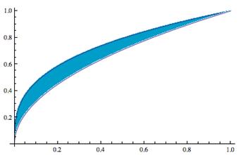
points of intersection of f and g, we set the two equations equal and solve. For example, find the area between the
functions ![]() and
and
![]() (see figure 8). Solving for where
f = g, we see that a = 0 and b = 1. Thus,
(see figure 8). Solving for where
f = g, we see that a = 0 and b = 1. Thus,
![]()
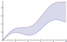
Figure 8
Graph of the Area Between the Functions
![]() and
and ![]()
See the examples in the Step-by-Step Explanation section for the complete solution.
In summary, the steps for solving an area-between-the-curves problem are as follows:
Graph the functions and consider the "rectangles" that would be set up and solve the problem.
Determine a and b (if necessary) and the points of intersection by solving
 for x.
Divide [a, b] into intervals if the functions intersect for values in [a, b] and determine which is the upper function on each interval so you can obtain positive differences when you remove the absolute values.
Set up the integrals and solve by finding and evaluating the antiderivatives.
Sum up the values and simplify as necessary.
See the Step-by-Step Explanation section for a detailed description of solving area-between-the-curves problems.