Population Growth
Step-By-Step Explanation
-
Example 1: Find the time constant for world population growth (assuming an exponential model with no factors limiting growth).
-
Example 2: Find the time constant for world population growth (assuming a logistic model with factors limiting growth).
Example 3: Analyze the interaction of two species in a predator-prey struggle inspired by a 1962 episode of The Twilight Zone.
Example 1
| Figure | Problem | |||||||||||||||||||||||||||||||||||||||||||||||||||||||||||||||||||||||||||||||||||||
|---|---|---|---|---|---|---|---|---|---|---|---|---|---|---|---|---|---|---|---|---|---|---|---|---|---|---|---|---|---|---|---|---|---|---|---|---|---|---|---|---|---|---|---|---|---|---|---|---|---|---|---|---|---|---|---|---|---|---|---|---|---|---|---|---|---|---|---|---|---|---|---|---|---|---|---|---|---|---|---|---|---|---|---|---|---|---|
|
Find the time constant (growth constant) for world population growth (assuming an exponential model). |
|||||||||||||||||||||||||||||||||||||||||||||||||||||||||||||||||||||||||||||||||||||
| Step | Equation | Explanation | ||||||||||||||||||||||||||||||||||||||||||||||||||||||||||||||||||||||||||||||||||||
1 |
| Data (which you can get from several sources, including the US Census Bureau) is needed to analyze the growth rate. Of course, data for periods of time before the twentieth century is estimated, as is some countries' world data. The data used herein is an average over these sources. |
||||||||||||||||||||||||||||||||||||||||||||||||||||||||||||||||||||||||||||||||||||
2 |
|
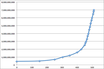
By inserting the data into Excel or a similar spreadsheet, we can generate a graph to visualize the data. Because Excel begins any graph at zero, the data was re-centered, with 1500 being the starting year, zero. Plotting the data shows the growth to be approximately exponential.
On this graph, the x-axis is relative to the year 1500. |
||||||||||||||||||||||||||||||||||||||||||||||||||||||||||||||||||||||||||||||||||||
3 |
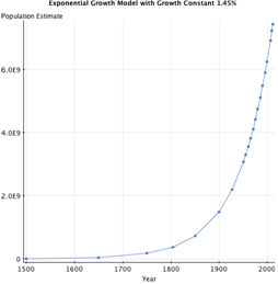
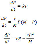
where P(t) is the world population at time t, P0 is the initial population, and k is the growth (time) constant. |
Assuming the exponential growth model given at left, let's see if we can determine a growth constant k that fits the data. |
||||||||||||||||||||||||||||||||||||||||||||||||||||||||||||||||||||||||||||||||||||
4 |
|
This model is the solution of the differential equation at left that results from the assumption that the population-growth rate is proportional to the size P(t) of the population at time t. Thus, the time (growth) constant k is the constant of proportionality from this assumption. Note that the time constant results from the proportionality constant of the equation at left. This constant is, in general, called the growth or decay constant. |
||||||||||||||||||||||||||||||||||||||||||||||||||||||||||||||||||||||||||||||||||||
5 |
That is, k is the relative (percentage) growth rate, which may be estimated using finite differences:
|
Solving this equation for k and using a discrete algebraic approximation gives us a way to estimate k. |
||||||||||||||||||||||||||||||||||||||||||||||||||||||||||||||||||||||||||||||||||||
6 |
|
In a spreadsheet like Excel, the differences may be calculated by defining a formula on the cells. The Relative Difference column of our table is the estimate of k. |
||||||||||||||||||||||||||||||||||||||||||||||||||||||||||||||||||||||||||||||||||||
7 |
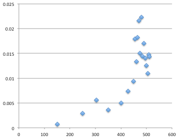
Number of Years |
Although the estimate for k seems to have varied greatly over the decades, it appears to average out to a value in the range of 0.013 to 0.016 over the past century. Plotting these values shows that the growth rate has been increasing (due to factors like, for example, the eradication of some diseases) but seems to be clustering from about 1950 forward (that is, t = 450 = 1950 − 1500 on the graph). It seems reasonable to make the estimation from this period because of the effects of modernization and technology. |
||||||||||||||||||||||||||||||||||||||||||||||||||||||||||||||||||||||||||||||||||||
8 |
|
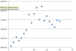
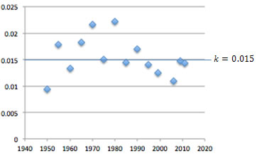
Zooming in on the data ("Year 0" is the year 1900 on the graph at left, with a horizontal time scale in decades) shows more clustering around the line k = 0.015. Averaging the data from 1900 forward gives a k value of 0.014 (that is, about a 1.4 percent growth rate). |
||||||||||||||||||||||||||||||||||||||||||||||||||||||||||||||||||||||||||||||||||||
9 |
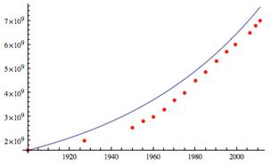
Graph Comparing Population Data (dots) and the |
Using Mathematica to plot the data against the model curve, however, shows that this estimate does not indicate a good fit. Although the data trends are the same as the exponential-growth model, the model drifts from the actual data, particularly from 1920 to 1960. |
||||||||||||||||||||||||||||||||||||||||||||||||||||||||||||||||||||||||||||||||||||
10 |
|
If we return to the graph in step 8, we see that the growth rate was increasing until around 1950, when it then seems to have clustered around k = 0.015. Let's consider analyzing the data since 1950. |
||||||||||||||||||||||||||||||||||||||||||||||||||||||||||||||||||||||||||||||||||||
11 |
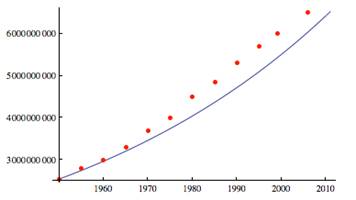
Graph Comparing the Population Data (dots) and the |
Averaging the values for k gives a value of approximately 0.0154. Plotting this model with our data, there appears to be a reasonable fit for our population data up to the mid-1960s to possibly 1970. However, errors remain from 1970 onward between the data and the model (see figure at left). Errors may occur because our averaging method may be flawed. Notice that the data points are not uniformly spaced in time. In particular, we have many more data points from 1990 forward; and these values may be more exact than the data estimates, especially in the period before 1900. |
||||||||||||||||||||||||||||||||||||||||||||||||||||||||||||||||||||||||||||||||||||
12 |
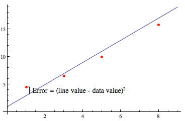
Linear Regression (Linear Least Square Fit) |
A more accurate method to estimate the time constant k is to use the method of linear least square fit, or as it is known in statistics, regression analysis. The regression-analysis method is the same as the linear least square fit methods covered in Calculus I, where the sum of the errors (squares of the values between a line and given data points) is minimized; that is,
|
||||||||||||||||||||||||||||||||||||||||||||||||||||||||||||||||||||||||||||||||||||
13 |
Graph of ln(ex) from x = 0 to x = 10
|
Recall from Calculus I that the line of least squares gives a best fit for approximately linear data. But our data is not linear (that is, it lies along an exponential function, not a linear one). There are regression methods based on fitting to arbitrary functions—minimizing the sum of errors between the data and a function—but another way is suggested if we notice that the log of the exponential is linear.
Notice that the time constant k corresponds to the slope of the linear function. |
||||||||||||||||||||||||||||||||||||||||||||||||||||||||||||||||||||||||||||||||||||
14 |
World Population Data Graphed on a Log Scale |
A technique in scientific study, where exponential growth and decay are common, is to plot the data on a log scale. Because we believe our population data to be exponential, let's plot it on a log scale (that is, the y-axis value is the log of the data value). |
||||||||||||||||||||||||||||||||||||||||||||||||||||||||||||||||||||||||||||||||||||
15 |
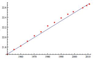
Graph of the Natural Log of the |
Now apply linear regression to the data. There are many tools for doing this (for example, the Analysis ToolPak in Excel or the StatCrunch program in MyMathLab), but here we will use the LinearModelFit function in Mathematica. Doing so gives a slope value of 0.0167874, which will correspond to the time constant k value. |
||||||||||||||||||||||||||||||||||||||||||||||||||||||||||||||||||||||||||||||||||||
16 |
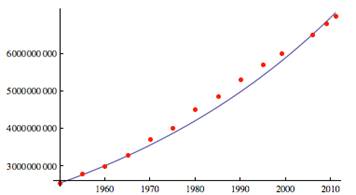
Data Graphed Against an Exponential Curve |
Plotting the exponential data with the exponential-growth model for k = 0.0167874 gives a better fit. (Note that the difference in the graphs in steps 15 and 16 is that one is the log and the other is the exponential model with the new k value.) |
||||||||||||||||||||||||||||||||||||||||||||||||||||||||||||||||||||||||||||||||||||
17 |
|
Calculating the doubling time based on this growth gives a value of about 41.3 years. That is, we would expect the world population to reach 14 billion people around 2053, assuming that the model and this rate of growth remains valid over that period of time. But there may be other limiting factors that affect this estimate. |
||||||||||||||||||||||||||||||||||||||||||||||||||||||||||||||||||||||||||||||||||||

Example 2
| Figure | Problem | |
|---|---|---|
|
Example 1 assumed a population-growth model with no restrictions, but what if there are limiting factors? For example, the amount of room and resources on our planet are finite, so how will these limiting factors affect population growth? Such factors are considered in the logistic model of population growth. Given a limiting population of 20 billion people and the growth rate determined in example 1, how long will it take for the population to reach 95 percent of its limit? |
|
| Step | Equation | Explanation |
1 |
|
In example 1, we assumed that the population would continue to grow with the determined growth constant and thus double in a little more than 40 years. But what if this is not the case? What if there is a limit on resources that will limit the growth to a maximum population of M people? A common assumption in population models is that k is determined by the relation k = r(M − P), where r > 0 is a constant (equivalent to the maximum growth rate) and M is the maximum value of the population size P. M is called the carrying capacity. Substituting into the growth model gives a new model equation called the logistic growth model, which is shown at left. |
2 |
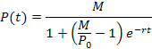
|
This model has the solution given at left. (This model is derived from methods of differential equations but can be verified by substitution.) |
3 |
|
Given that the seven-billionth person was born in 2012, let P0 be 7 (billion) and M = 20. Also assume that the growth rate does not increase so that r is equal to the k value found in example 1 above. |
4 |
|
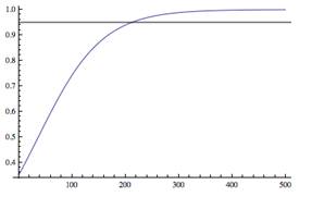
Graphing our logistic solution (the graph at left graphs P(t) as a percentage of the assumed carrying capacity M = 20) indicates that the 95 percent level will be reached in a little more than 200 years. Solving the problem algebraically gives 212 years. |
5 |
|
Our solution shows that without other intervening factors, humankind will reach 95 percent of Earth's capacity in a little more than 200 years—a blink in cosmic time. But this result is based on an assumption that the planet's carrying capacity is 20 billion people. Is that assumption correct? The global population reached a billion around 1800, just a couple of years after Thomas Malthus published his famous essay, warning that human numbers would always be held in check by war, pestilence, or "inevitable famine," which were the assumptions for his model. Finding a way to test the truth of our assumptions may be the most difficult part of any mathematical model. |

Example 3
| Figure | Problem |
|
As we have seen in examples 1 and 2, the world population is growing exponentially and seems limited only if we assume a maximum carrying capacity. What if science fiction becomes science fact and humans become the prey of extraterrestrials? For example, see the Damon Knight short story (or the associated Twilight Zone television series episode) "To Serve Man," whose title is a play on the word serve. In this case, it may be appropriate to use a predator-prey model in which the population size of the prey may vary with unfortunate interactions with the predator, which itself may have population variation due to the amount of available prey. Assume that 200,000 people-eating aliens from outer space show up in 2012 after a long journey. They decide Earth is a good place to live and that humans make good prey and an appealing food supply. Furthermore, due to their advanced technology, the aliens cannot be killed by the humans and thus die only from natural causes or starvation. Also assume that, although the aliens have a long life span (say, 200 years), their growth rate is low (assume ka = 0.003). Qualitatively analyze the interaction of the two species. |
|---|---|---|
| Step | Equation | Explanation |
1 |
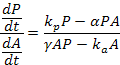
where P(t) is the human population at time t, A(t) is the alien population, kp and ka are their respective growth constants, and ∝ and γ are the interaction constants. |
Given the assumptions, it seems reasonable to use the Lotka-Volterra extension of the Kolmogorov predator-prey model. The Lotka-Volterra model makes the following assumptions:
|
2 |
ka = 0.003 |
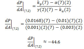
From example 1, we have kp = 0.0168, and we are given ka = 0.003. Assume that ∝ and γ are 0.01 and 0.001, respectively. |
3 |
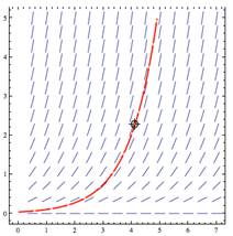
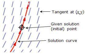
The blue lines represent the tangent line directions (slopes) |
Because the analytic solution of these equations is beyond the scope of this course, let's take a different approach. We can gain insight into the solution using qualitative methods, such as a slope field. A slope field is a graph of the tangent directions at "each" point of the xy plane. That is, from the differential equations, a formula for the tangent lines at a point (x, y) is determined, and the tangent slopes are drawn as line segments on some grid of points (see the diagram at left). |
4 |
|
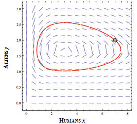
The diagram at left shows a "zoomed" view of the previous diagram. The arrows on the (red) solution curve indicate the direction with increasing time. |
5 |
|
To draw the tangent line directions in the slope field, we must determine the derivative dp/dA from the differential equations. We can do this by "dividing the equations" and "dividing out" dt. We could make this determination mathematically precise by using limits; but for our discussion, we will assume it can be done. |
6 |
|
Thus, for any value pair (P, A), we can calculate the slope of the tangent line. For example, at the initial condition point, (P, A) = (7, 2), where P is in billions of people and A is in hundred-thousands of aliens, the slope of the tangent is approximately −44.6. |
7 |
|
Because the solution must initially follow this tangent direction, it is bad news for humankind because the population of people will start dropping immediately due to interactions with the aliens, and the now well-fed alien population will increase. |
8 |
|
Over time, the human population dramatically decreases but does not fall below about 1 billion. As the human population drops below 2 billion, the alien population begins to drop as food interactions become less frequent. Finally, the human population begins to rise, along with a slow growth (upward tend) in the alien population. This pattern then falls into a cyclic behavior. Notice that the human population never grows beyond a little under 8 billion and the alien population never grows beyond 250,000. |
9 |
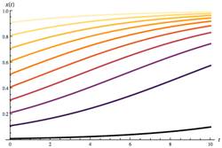
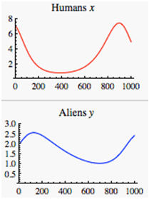
|
These graphs, derived from the phase plane, show the period cycle of the populations over a 1,000-year period. |
10 |
Stationary (or fixed) point solution of the Lotka–Volterra equations: |
Finally, notice in the slope-field diagram in step 8 that the parametric solution curve seems to orbit about a central point. This is indeed the case, and this point is called the stationary (solution) point of the equations. It is given by the ordered pair at left. So if the aliens had arrived on Earth with a population of 168,000 and found a human population of 3 billion, the population values would never change—that is, the human population would be enough to feed the aliens and never diminish in number. |


Works Consulted
Cohen, J. E. (1995). How many people can the Earth support? New York: Norton.
Negative Population Growth. (2012). Total midyear world population, 1950–2050. Retrieved from http://www.npg.org/facts/world_pop_year.htm.
Population Reference Bureau. (2012). The faces of unmet need. Retrieved from http://www.prb.org/.
Rosenberg, M. (2012). Current world population: Current world population and world population growth since the year one. About.com Geography. Retrieved from http://geography.about.com/od/obtainpopulationdata/a/worldpopulation.htm.
Wikimedia Foundation. (2012). World population. Wikipedia. Retrieved from http://en.wikipedia.org/wiki/World_population.
Worldometers. (2012). World population clock. Retrieved from http://www.worldometers.info/world-population/.