Population Growth
Summary
According to US Census Bureau's (2012) estimates, the seven-billionth person on Earth was born sometime around April Fool's Day of 2012. It is important to analyze various population models and population growth to better understand our planet and its limited natural resources.
The Exponential-Growth Model
The generally accepted population model assumes that, without constraints, the growth rate (derivative of the population with respect to time) is directly proportional to the size of the population at time t; that is,
![]()
where k is a constant called the relative growth rate and P(t) is the population at time t. Equation (1) is called a differential equation because it involves a function and its derivative.
Solving for k in equation (1), we have
Equation (2) tells us that the relative growth rate k (the growth rate dP/dt divided by the population P) is, in fact, constant. That is, according to equation (2), a population with a constant relative growth rate must grow exponentially.
The solution to equation (1) is, in fact, the exponential-growth equation (3), which we use to model population growth:
![]() ,
,
where P(0) = P0 is the population at time equal to zero, called the initial population.
Note that this problem can be solved analytically, using differentials:
![]()
Integrating gives
![]()
which converts to the exponential equation
![]()
The constant was determined by substituting t = 0, which gave ec = P(0), the initial population.
The value of the growth constant k is associated with the "doubling time" (the amount of time required to double the initial population) given by,
![]()
In business, this doubling-time relationship is approximated by the "Rule of 72" for compound-interest problems, where the doubling time is given by 72 divided by the interest rate as a percentage to determine the amount of time required to approximately double an initial investment.
We may ask, what is the doubling time of the world population? Using population data from 1500 to 2010 CE, a graph of the data shows the growth to be approximately exponential.
Figure 1
World Population Appears to Be Growing at an Exponential Rate
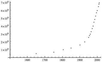
In fact, using an exponential function with k = 0.017, as derived in the examples in the Step-by-Step Explanation section, gives a curve that fits the data very well. For this value of k, the world population would double approximately every 40 years:
![]()
Thus it appears that the world population is currently growing at a rate of approximately 1.7 percent, which indicates that it will double to more than 14 billion people in another 41 years (i.e., around 2050). The exponential-growth model seems fairly accurate because people have no real predators.
Of course, the above calculation assumes that the exponential-growth rate can and will be maintained, but was Thomas Malthus correct? Will issues like limited natural resources come into play? Such factors are more effectively modeled using a logistic model of population growth.
The Logistic Model
The human population, with no true predator, may be limited instead by resources—the size of the planet, ability to grow enough food, and so forth. These situations are best modeled by the logistic equation (sometimes called the Verhulst model or logistic growth curve), which is a model of population growth first published by Pierre Verhulst around 1845. The model is continuous in time and is described by the differential equation,
![]()
where r is the rate of maximum population growth (sometimes called the Malthusian parameter) and K is the carrying capacity—that is, the maximum sustainable population growth. This equation can be rewritten in the form,
![]()
where x is defined as ![]() . This equation is called the logistic equation and has the solution,
. This equation is called the logistic equation and has the solution,

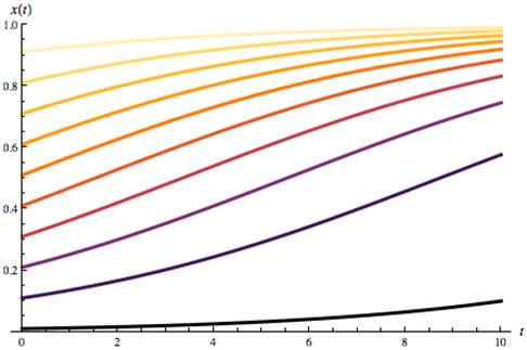
The parameter r is usually taken to be positive. Figure 2 shows some plots for r positive and various initial conditions x0. The graphs show, for various initial starting points, how the population "levels off" over time.
Figure 2
Solutions to the Logistic Equation for r = 0.25
The Predator-Prey Model
Predator-prey models involve two interacting populations (or species), where one is a predator, killing and perhaps feeding off another population, called the prey (the interaction of foxes and rabbits is a good example of this model). If two populations whose sizes at a reference time t are respectively denoted by x(t), y(t), then a general model of interacting populations may be written in terms of two autonomous (that is, time does not appear as an explicit variable) differential equations:
![]()
![]()
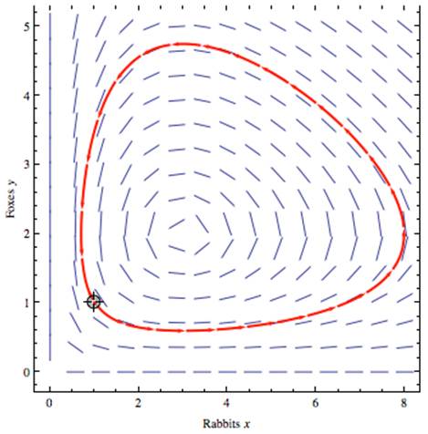
where a and b are population-growth constants and the two xy terms model the interaction of the two species (controlled by constants p and r). Although this system of two equations is difficult to solve, a qualitative representation (called a phase-plane diagram) can be constructed, as shown in figure 3.
The graph in figure 3 is a qualitative representation of a solution to the predator-prey model. The line segments represent the populations' rate of change, thus their growth must follow these tangent lines. The red curve with a given initial condition shows how the populations will become cyclic—each growing and diminishing over time.
Figure 3
Qualitative Representation of a
Solution to the (Kolmogorov) Predator-Prey Model
Reference
United States Census Bureau. (2012). U.S. and world population clocks. Retrieved from http://www.census.gov/main/www/popclock.html.